Maple/Octave Implementation of Classification Using Logistic Regression:
Main Routine:
data = load('datalogisticregression.txt');
X = data(:, [1, 2]); y = data(:, 3);
rf=100;
X = [X , X.^2/rf, X(:,1).*X(:,2)/rf];
pos = find(y==1); neg = find(y==0);
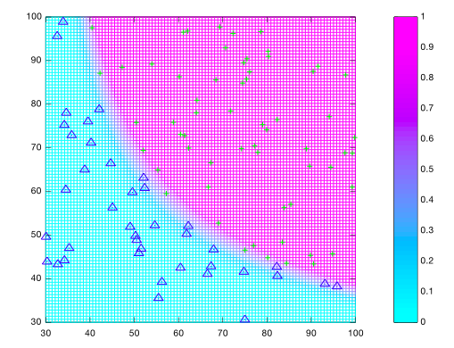
plot(X(pos,1),X(pos,2),'g+',X(neg,1),X(neg,2),'bo','MarkerSize',8);
hold on
[m, n] = size(X);
X = [ones(m, 1) X];
init_theta = zeros(n + 1, 1);
[cost, grad] = costfunction(init_theta, X, y);
options = optimset('GradObj', 'on', 'MaxIter', 1000);
[theta, cost] =
fminunc(@(t)(costfunction(t, X, y)), init_theta, options);
fprintf('After optimization cost is: %f\n',cost);
fprintf('Parameter Vector is:\n');
theta
prob = sigmoid([1 50 80 50^2/rf 80^2/rf 50*80/rf] * theta);
fprintf('For feature 45 and 80, probability is %f\n', prob);
prediction = sigmoid(X*theta) > 0.5;
fprintf('Training Accuracy: %f\n', mean(double(prediction == y)) * 100);
X1 = linspace(30,100,100)';
X2 = linspace(30,100,100);
z = zeros(100,100);
z = sigmoid(1.0*theta(1) + X1*ones(1,100)*theta(2) + ones(100,1)*X2*theta(3) +
(X1*ones(1,100)).^2/rf*theta(4) + (ones(100,1)*X2).^2/rf*theta(5) +
theta(6)*X1*X2/rf);
mesh(X1',X2,z);
colormap cool;
colorbar;
print -dpng regplot.png
hold off
Sigmoid Function:
function g = sigmoid(z)
g = 1./(1+exp(-z));
end
Cost Function:
function [J, grad] = costfunction(theta, X, y)
m = length(y);
J = 0;
grad = zeros(size(theta));
J = (-y'*log(sigmoid(X*theta)) - (1-y')*log(1-sigmoid(X*theta)))/m;
grad = (X'*(sigmoid(X*theta)-y))/m;
end
Data File:
[datalogisticregression.txt]