Numerical Relativistic Hydrodynamics
Hydrodynamics allows for an effective description of macroscopic matter
providing the matter is in local
thermal equilibrium.


 Therefore
the state of a patch of fluid is fully described by a set
of position dependent state variables (i.e. fields).
The evolution of these fields is governed by the relativistic Euler's
equations.
In addition to the equations of motion one must supply the
eqaution of state. The equation of state for the ideal fluid has the
form
where
is the isotropic pressure is the rest mass
density and is the specific internal energy. is the adiabatic index ().
Euler's equations constitute a set of hyperbolic partial differential
equations.
By specific choice of variables these equations can be written in
conservative form (possibly with sources).
It is well known that solutions of the Euler's equations generically
develop discontinuities even from initially smooth data.
One can either smooth the discontinuities by introducing an artificial
viscosity or use a different method for solving the hydrodynamic
equations - the so called high resolution shock capturing methods
(HRSC). In recent years the latter approach became increasingly more
popular. HRSC methods are based on a different type of discretization -
the
so-called finite volume discretization. Here instead of approximating
the value of a field variable at a grid point one evolves the volume
average
of the field over a computational cell. One then calculates the
fluxes of the conservatives fluid variables over all of the cell
boundaries
and then adjusts the cell averages accordingly (if sources are
present their contribution is also included)
Since the Einstein equations are most often solved with finite
difference approximation it is not straightforward to incorporate
matter into the calculations. I am currently involved in a
collaborative effort with Frans Pretorius to include the HRSC hydro
solver into his parallel adaptive mesh refinment infrastructure
(PAMR/AMRD). More about this can be found here.
Therefore
the state of a patch of fluid is fully described by a set
of position dependent state variables (i.e. fields).
The evolution of these fields is governed by the relativistic Euler's
equations.
In addition to the equations of motion one must supply the
eqaution of state. The equation of state for the ideal fluid has the
form
where
is the isotropic pressure is the rest mass
density and is the specific internal energy. is the adiabatic index ().
Euler's equations constitute a set of hyperbolic partial differential
equations.
By specific choice of variables these equations can be written in
conservative form (possibly with sources).
It is well known that solutions of the Euler's equations generically
develop discontinuities even from initially smooth data.
One can either smooth the discontinuities by introducing an artificial
viscosity or use a different method for solving the hydrodynamic
equations - the so called high resolution shock capturing methods
(HRSC). In recent years the latter approach became increasingly more
popular. HRSC methods are based on a different type of discretization -
the
so-called finite volume discretization. Here instead of approximating
the value of a field variable at a grid point one evolves the volume
average
of the field over a computational cell. One then calculates the
fluxes of the conservatives fluid variables over all of the cell
boundaries
and then adjusts the cell averages accordingly (if sources are
present their contribution is also included)
Since the Einstein equations are most often solved with finite
difference approximation it is not straightforward to incorporate
matter into the calculations. I am currently involved in a
collaborative effort with Frans Pretorius to include the HRSC hydro
solver into his parallel adaptive mesh refinment infrastructure
(PAMR/AMRD). More about this can be found here.
In some cases one can assume that the fluid is not
coupled to gravity (a test fluid) and only moves in a prescribed
geometry. This geometry is typically a static or stationary solution of
Einstein's eqautions such as Minkowski, Schwarzschild or Kerr
spacetime.
This approach has been successfully used to simulate astrophysical
jets,
wind accretion onto black holes and accretion disc around black holes.
In order to familiarize myself with the HRSC methods in the framework
of GR
I have developed a code which can evolve relativistic ideal fluid in a
background geometry in 1D,2D (spherical symmetry, axisymmetry) and 3D.
The code can run in a parallel environment (using PAMR) and performs
well on a Linux Beowulf cluster.
Astrophysical Jets
Jets are ubiquitous in extragalactic radio sources associated with
active galactic nuclei. Although to explain their origin GR
magnetohydrodynamics is needed, to study the morphology of the jet a SR
hydrodynamics is sufficient. The following is a simulation of a 2D
planar
jet (
 ) moving
through
an extragalactic medium (
) moving
through
an extragalactic medium (
 ).
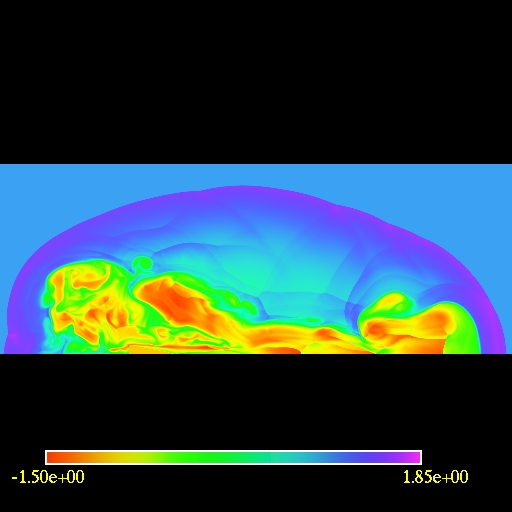
The first image/movie below shows the log of the fluid density of a the
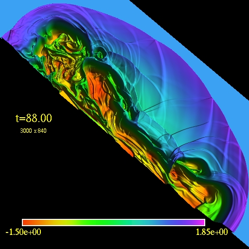
jet. The second image/movie shows a 3D view of the domain. In order to
visualize the fluid flow one can trace test particles
trajectories.
I started with random uniform particle distribution and regularly added
particles into the jet source. The third image/movie shows the motion
of the
tracers.
Since the jet is symmetric it is sufficient only to use half of the
domain for calculations and to use reflection boundary conditions at
the symmetry axis.
The computational domain is (-20,55)x(0,21) and the resolution is
3000x840 cells.
).
The first image/movie below shows the log of the fluid density of a the
jet. The second image/movie shows a 3D view of the domain. In order to
visualize the fluid flow one can trace test particles
trajectories.
I started with random uniform particle distribution and regularly added
particles into the jet source. The third image/movie shows the motion
of the
tracers.
Since the jet is symmetric it is sufficient only to use half of the
domain for calculations and to use reflection boundary conditions at
the symmetry axis.
The computational domain is (-20,55)x(0,21) and the resolution is
3000x840 cells.
Note the presence of an external bow shock and the vortices due to
the Kelvin-Helmholtz instability.
 |
 |
 |
2D view of the
computational
domain. Logarithm of the fluid density is plotted.
(click to play mpeg movie)
|
3D view of the
computational
domain. Logarithm of the fluid density is plotted.
(click to play mpeg movie) |
Visualization of
the fluid flow by trace particles.
(click to play mpeg movie)
|
Wind Accretion onto Black Hole
These are the results of simulations of
a relativistic wind accretion onto a Schwarzschild BH. The models are
taken from the paper by Font et. al.
A
NUMERICAL STUDY OF RELATIVISTIC BONDI-HOYLE ACCRETION ONTO A MOVING
BLACK HOLE:AXISYMMETRIC COMPUTATIONS IN A SCHWARZSCHILD
BACKGROUND,494,297-316 (1998)
Here is the table from the paper describing the models (I think that rmin(ra)
for model MC2 should be 0.57 - 0.44 would be below the Schwarzschild
radius)
TABLE 1
INITIAL MODELS
| Model |
cs∞ |
G |
Μ∞ |
v∞ |
ra(M) |
rmin(ra) |
rmax(ra) |
tf(M) |
| MA1... |
0.1 |
1.1 |
1.5 |
0.15 |
30.8 |
0.125 |
10.0 |
4000 |
| MA2... |
0.1 |
1.1 |
5.0 |
0.5 |
3.8 |
0.57 |
10.0 |
750 |
| MB1... |
0.1 |
4/3 |
1.5 |
0.15 |
30.8 |
0.125 |
10.0 |
4000 |
| MB2... |
0.1 |
4/3 |
5.0 |
0.5 |
3.8 |
0.57 |
10.0 |
750 |
| MC1... |
0.1 |
5/3 |
1.5 |
0.15 |
30.8 |
0.125 |
10.0 |
2000 |
| MC2... |
0.1 |
5/3 |
5.0 |
0.5 |
3.8 |
0.44 |
10.0 |
750 |
| UA1... |
0.31 |
1.1 |
1.5 |
0.47 |
3.2 |
0.69 |
9.38 |
200 |
| UA2... |
0.31 |
1.1 |
3.0 |
0.93 |
1.04 |
2.12 |
28.85 |
110 |
| UB0... |
0.57 |
4/3 |
0.6 |
0.34 |
2.2 |
1.0 |
13.64 |
200 |
| UB1... |
0.57 |
4/3 |
1.5 |
0.86 |
0.92 |
2.39 |
32.61 |
200 |
| UC0... |
0.81 |
5/3 |
0.6 |
0.49 |
1.1 |
2.0 |
27.27 |
200 |
| cs∞ |
asymptotic sound speed
(i.e., at the outer boundary)
|
| G |
adiabatic exponent
|
| Μ∞ |
asymptotic Mach number at
infinity
|
| v∞ |
asymptotic flow velocity
|
| ra(M) |
accretion radius
|
| rmin(ra) |
inner boundary in units of
accretion radius
|
| rmax(ra) |
outer boundary in units of
accretion radius |
| tf(M) |
final time at which the
simulation was stopped |
|
 |
|
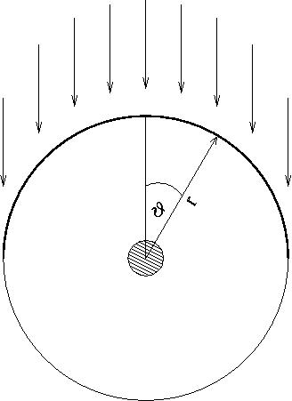
Wind accreation schematics.
The outer circle is the outer boundary. The small circle in the
middle represents the inner boundary with the black hole.
|
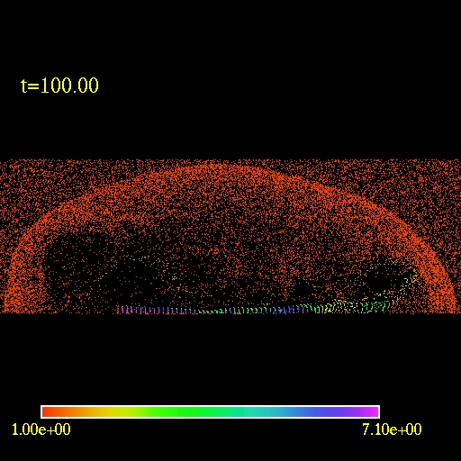
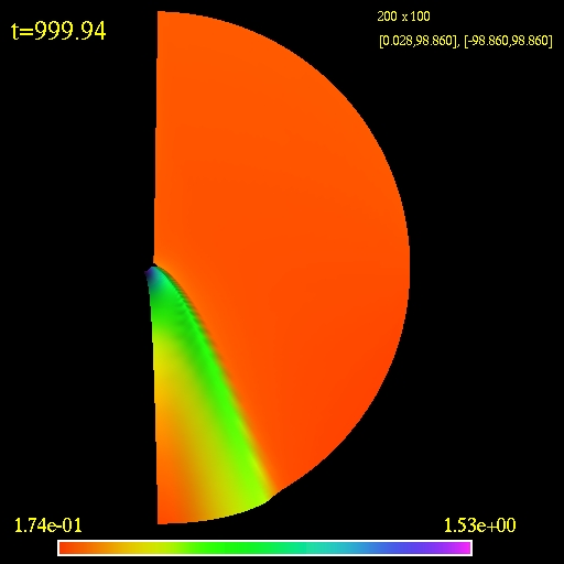
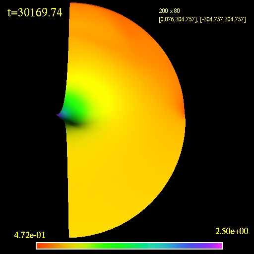
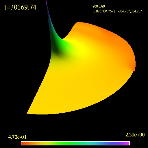
First is the simulation of the model MC2 performed on a 200x100 grid
(r,theta) using Eddington-Finkelstein ingoing coordinates. The grid is
logarithmic in r-direction and uniform in theta. The inner radius is
located at r=1.75M and the outer radius is at r=100M. In this
simulation
(unlike in the paper) I put vacuum in the whole domain except at the
ghost zones in the upper hemisphere at initial time. The vacuum was a
true vacuum, i.e., all the variables were set to zero. It is a bit
tricky to evolve such a setup but the method I implemented seemed to
work fine. Since this is log10 plot I added 1.e-3 to the
density so vacuum would be represented by the value -3.
|
 |
| 2D view of the computational
domain. Logarithm of the fluid density is plotted.
(click to play mpeg movie) |
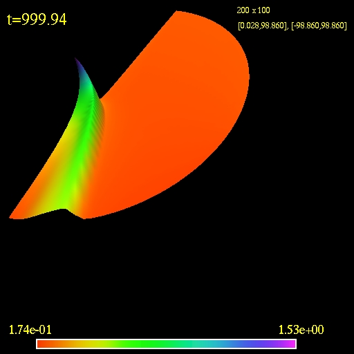
3D view of the computational
domain. Logarithm of the fluid density is plotted.
(click to play mpeg movie)
|
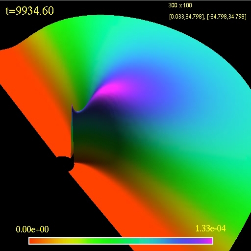
The next simulation is for the model
MB1. This particular one is done in Schwarzschild coordinates but the
results do not change when using Eddington-Finkelstein ingoing
coordinates. The simulation shows that if a stationary state is reached
it would be qualitatively different than the one for the model MC2
which
is unexpected. I performed many simulations in both types of coordinate
systems with different resolutions, domain sizes and flux
approximations. All result in the same behaviour, i.e., the
detachment of the initially formed shock and its dispersion. My
computed
accretion rates for all tested models agree to those published until
the tf(M) for each
simulation. My evolution of the model MC1 shows similar behaviour
- a hint of it might be even present in the paper - the simulation of
C1 shows a detached shock but the simulation was stopped at t=2000M.
|
 |
2D view of the computational
domain. Logarithm of the fluid density is plotted.
(click to play mpeg movie)
|
3D view of the computational
domain. Logarithm of the fluid density is plotted.
(click to play mpeg movie)
|
Accretion Discs
The most spectacular accretion discs in
nature are found in active
galactic nuclei
and most probably at the center of quasars.
It is thought that a super massive black hole is located at the center
with matter orbiting around it and spiraling inwards. Below are two
simulations of accretion discs around Schwarzschild black hole.
The first image/movie shows an evolution of an stable accretion disc.
All of the matter is inside its Roche lobe so no matter transfer should
occur (a "numerical leak" can be seen at the end of the simulation).
The second image/movie shows an evolution of a disc overflowing its
Roche lobe. There is a steady matter flow into the black hole. The
model s are taken from
arxiv:astro-ph/0203403.

|
 |
3D view of the computational
domain. Logarithm of the fluid density is plotted.
(click to play mpeg movie)
|
3D view of the computational
domain. Logarithm of the fluid density is plotted.
(click to play mpeg movie)
|