Critical Phenomena in Gravitational
Collapse
Critical phenomena in gravitational collapse were discovered by
Choptuik in 1993 in the spherically symmetric collapse of massless
scalar field. Since then the phenomenon has been
observed in a variety of matter sources.
At the threshold of gravitational collapse the matter is just
about to form a black hole and an infinitesimally small perturbation
can either cause the matter to disperse to infinity or to form a black
hole.
The dynamics close to the threshold exhibits interesting behaviour
such as power law scaling of length scales, self similarity of the
solutions and universaity. A typical setup is to take an initial matter
distribution parametrized
by a single parameter
 . Then one performs a bisection
search to determine the critical value
. Then one performs a bisection
search to determine the critical value
 .
The critical exponent can be determined from the scaling relation of
the black hole mass
or, more conveniently,
from the scaling relation of the
maximum of the scalar curvature
.
The critical exponent can be determined from the scaling relation of
the black hole mass
or, more conveniently,
from the scaling relation of the
maximum of the scalar curvature
To numerically evolve near critical solutions is a non-trivial task.
The critical solution is self-similar, i.e., it repeats itself
on ever decreasing length scales. The fluid density and pressure
increase by many order of magnitudes and in some cases the
fluid velocity becomes extremely relativistic.
Critical collapse is a very good starting point for getting acquinted
with advanced numerical techniques such as adaptive mesh refinment
(AMR).
A widely studied matter model is the ultrarelativistic limit of ideal
fluid
with the equation of state
where
 is the total
energy density of the fluid.
I was in particularly interested in the limit of
is the total
energy density of the fluid.
I was in particularly interested in the limit of
 in which the fluid becomes dust-like.
The dust limit is interesting to study since it has been conjectured
that the scaling exponent for dust should
assume some simple value such as 1. Also there have been claims of
naked singularity formation in ideal fluid collapse for
in which the fluid becomes dust-like.
The dust limit is interesting to study since it has been conjectured
that the scaling exponent for dust should
assume some simple value such as 1. Also there have been claims of
naked singularity formation in ideal fluid collapse for
 .
Another way of investigating the critical collapse is to use the fact
that the critical solution is continuously selfsimilar.
By using the selfsimilar ansatz the set of PDEs transform into a set of
ODEs
that can then be solved quite easily numerically to a very high
precision
(therefore I will call it exact).
One then performs a perturbation analysis around the critical solution
to determine the scaling exponent.
.
Another way of investigating the critical collapse is to use the fact
that the critical solution is continuously selfsimilar.
By using the selfsimilar ansatz the set of PDEs transform into a set of
ODEs
that can then be solved quite easily numerically to a very high
precision
(therefore I will call it exact).
One then performs a perturbation analysis around the critical solution
to determine the scaling exponent.
 Below
are some results from the numerical calculations.
For the numerical simulations we used spherical polar coordinates
with the metric element
The
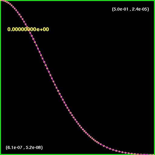
first image/movie shows the initial profile of the fluid density.
The evolution can be seen by clicking on the image.
The evolution is shown in the standard coordinate.
Also note that the magnitude increases by a factor of 107.
The second image shows a near-critical solution of
Below
are some results from the numerical calculations.
For the numerical simulations we used spherical polar coordinates
with the metric element
The
first image/movie shows the initial profile of the fluid density.
The evolution can be seen by clicking on the image.
The evolution is shown in the standard coordinate.
Also note that the magnitude increases by a factor of 107.
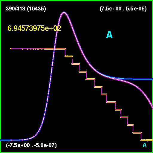
The second image shows a near-critical solution of
 compared with the exact one.
This image and the movie are shown in self similar coordinates.
The stairs-like line represents a grid hierarchy level. At each
successive
hierarchy level the distance between two neighbouting points is
reduced by a factor of two.
The grid hierarchy is adjusted whenever certain criteria are not met.
In that case the calculation starts from a previous
(successful) checkpoint with adjusted grid structure.
This scheme assures that our preset criteria are satisfied during the
entire evolution.
compared with the exact one.
This image and the movie are shown in self similar coordinates.
The stairs-like line represents a grid hierarchy level. At each
successive
hierarchy level the distance between two neighbouting points is
reduced by a factor of two.
The grid hierarchy is adjusted whenever certain criteria are not met.
In that case the calculation starts from a previous
(successful) checkpoint with adjusted grid structure.
This scheme assures that our preset criteria are satisfied during the
entire evolution.
Note that the numerical and exact solutions match only in a limited
region and have very different behaviour asymptotically.
This is due to the fact that the exact solution represents spacetime
that is not asymptotically flat, whereas in the
numerical calculations there is only a finite amount of matter and the
resulting spacetime is asymptotically flat.
However, the scaling exponent only depends on the behaviour
near to the origin where the both solution match.
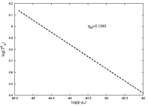
The last image shows data points obtained from numerical
simulations together with the linear fit and the value of the scaling
exponent.
More details can be found in the paper
Critical Colapse of an
Ultrarelativistic Fluid in the
 Limit
(gr-qc/0508062)
Limit
(gr-qc/0508062)
|
 |
Initial density profile of the
fluid density in standard spherical polar coordinate
 .
.
(click to play mpeg movie) |
Comparison of the numerical and
exact critical solutions of
 in self-similar
coordinates.
in self-similar
coordinates.
The hierarchy levels are also shown.
(click to play mpeg movie)
|
|
 |
|
Data obtained from subcritical
runs for
 .
The line represents the best linear fit to the data. The value of the
scaling exponent obtained from the linear fit is
.
The line represents the best linear fit to the data. The value of the
scaling exponent obtained from the linear fit is

|