Brans-Dicke / Massless Scalar Field Critical Solutions M.W. Choptuik and S.L. Liebling, August 2007

Description of Numerical Experiments

Using overlapping ingoing Gaussian pulses for both the Brans-Dicke (xi(t,r)) and massless scalar (phi(t,r)) fields, and with the Brans-Dicke coupling parameter, omega, fixed at omega = 10.0, a sequence of critical solutions, labelled 0, 1, 2, 3, 4, 5 and 6 below, was generated. Initial data for solution 0 had phi(0,r) = 0, in which case the model reduces to a massless scalar field in general relativity (phi(t,0) remains identically 0 throughout the evolution). Initial data for solution 6 had xi(0,r) = 0, but a non-zero xi(t,r) then develops dynamically. Solutions 1, 2, 3, 4 and 5, then, roughly interpolate between the two extremes, with the contribution of phi to the critical solution monotonically increasing with increasing solution number. In addition, another two runs were performed in which xi(0,r) was always fixed to 0, and the form of the initial scalar field was also fixed, but where omega = 1.0 and omega = 100.0 were used.

The first screenshot below shows central (r=0) values of the two fields, phi(t,0) and xi(t,0), with a time axis (x-axis) in which instants of time that are roughly equidistributed in ln(t* - t) are labelled 1, 2, ..., 300, 301.  In each frame, the magenta line is phi(t,0), the cyan line is xi(t,0), and the x-axis (phi, xi = 0) is shown in red. Also, solutions are "increasingly critical" as one pans from left to right in each plot.

There is thus some indication from these plots that, at least for omega=10.0 (and presumably for other values of omega in the DSS regime), each effective "relative admixture" of phi and xi leads to a distinct critical evolution for each of the two fields and that the "parity" of either of the fields w.r.t. Delta/2 is indeterminate except for the case where phi identically vanishes. Note, however, that the geometry in each case is apparently identical to the original massless scalar echoer, at least as far as our numerics can tell us. Evidence for this last statement can be seen in the second screenshot, which shows dm/dr(t**,r) vs ln(r) for each of the near-critical solutions, where t** ~ t*, and where m(t,r) is the (total) mass-aspect function.  The last plot shows the superposition of the 6 solutions (with NO rescaling or shifting of data) for the x-axis range -8.0 < ln(r) < 0.85.

Further, the third screenshot shows that, for fixed initial weighting of the two fields, the distribution of the field at criticality is likely to be omega-dependent. The three frames show the same quantities plotted in the first screenshot, with each critical solution being generated with xi(0,r) = 0, and with omega varying as indicated.

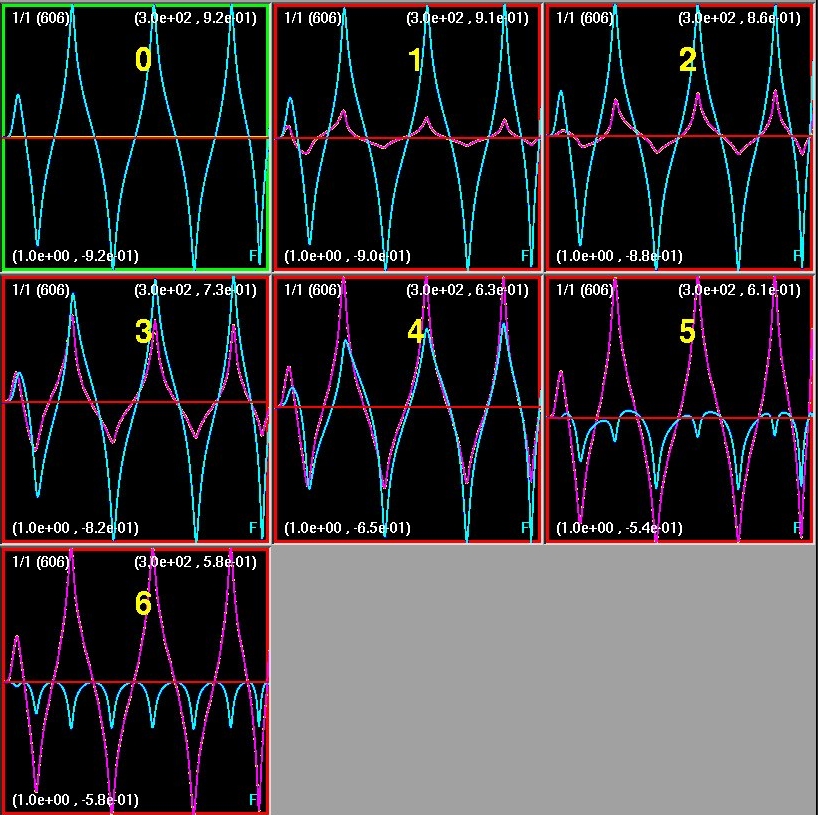
Screenshot 1: Central value of fields in near critical evolutions with varying contributions of Brans-Dicke (cyan) and massless (magenta) scalars.

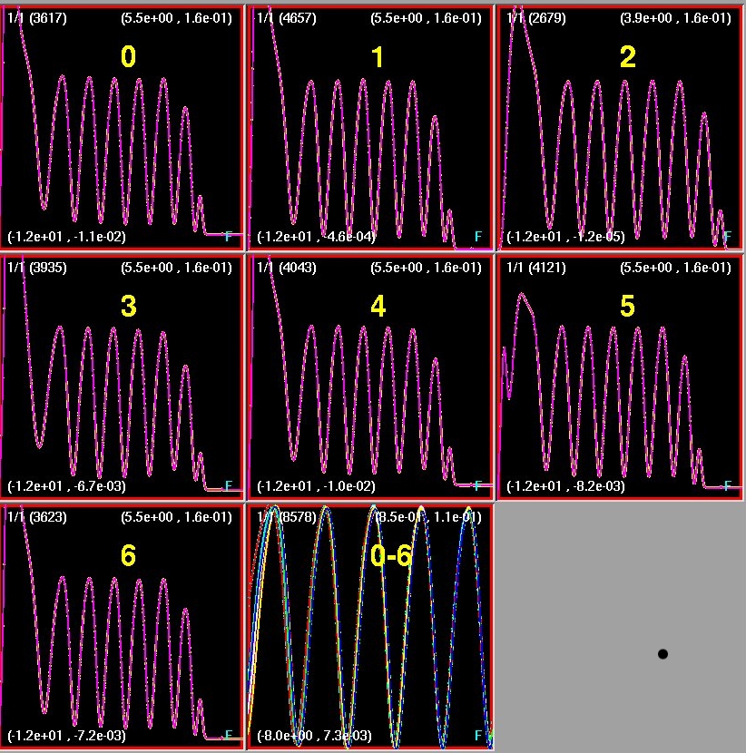
Screenshot 2: Late time snapshot of dm/dr(t**,r) for near critical evolutions as above.

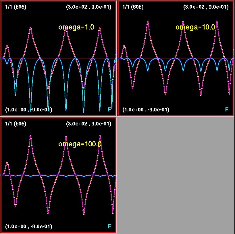
Screenshot 3: Central value of fields in near critical evolutions, all with xi(0,t) = 0, and with omega varying as indcated.  Cyan: Brans-Dicke field.  Magenta: Massless scalar field. Red: x-axis

Maintained by choptuik@phas.ubc.ca. Supported by CIFAR, NSERC, CFI, BCKDF and UBC.